Chapter 3 - Numerical modelling#
Important
NOTES ABOUT CHAPTER 3
The exercises in this chapter will be graded on the following criteria: (1) does the program run? (2) Does it do the right thing as specified in assignment and is it properly commented (3) Do your answers show insights into the models? See the end of this chapter for the full rubric.
You will receive an individual grade based on the competency of your coding and understanding of how this code relates to reality.
There are 3 exercises that you must hand that increase in difficulty and required time for completion.
Try to schedule your workload accordingly.
Please note for this exercise you must submit the scripts (with appropriate comments) as .zip file which will be used to determine your grade.
More important however is the Word document or PDF with your answers and explanations. This document should be accompanied by a number of screenshots of the modelling results.
The deadline for this Chapter is at 9:00 before the start of next practical.
3.1 A very simplified morphodynamic model#
In this section we consider a one-dimensional river with an initial constant slope \(S_0 = -0.1\) m/m. To gain insight, we want to compute the evolution of the river bed in space and time using very basic physical laws. Similar approaches are used in cellular automats of rivers and in so-called reduced-complexity models in earth surface, processes and landforms (try a search in Google Scholar to see debates and controversies). In this model, we do not consider the influence of the water motion and critical Shields number etc. on sediment transport. The total sediment transport rate \(q_t\) [in \(m^3\ s^{-1}\) per m width, or \(m^2\ s^{-1}\)] is therefore assumed to depend simply linearly on the local bed slope \(S\). More precisely, we assume that: In this section we consider a one-dimensional river with an initial constant slope \(S_0 = -0.1\) m/m. To gain insight, we want to compute the evolution of the river bed in space and time using very basic physical laws. Similar approaches are used in cellular automats of rivers and in so-called reduced-complexity models in earth surface, processes and landforms (try a search in Google Scholar to see debates and controversies). In this model, we do not consider the influence of the water motion and critical Shields number etc. on sediment transport. The total sediment transport rate \(q_t\) [in \(m^3\ s^{-1}\) per m width, or \(m^2\ s^{-1}\)] is therefore assumed to depend simply linearly on the local bed slope \(S\). More precisely, we assume that:
where \(\alpha_{s_t}\) is a proportionality coefficient (with the same unit as sediment transport) of the total sediment transport.
To solve this problem numerically, it needs to be discretized in space and in time. The reach of the river under consideration, of length \(L\), is divided into \(Nx\) sub-reaches, or grid cells, of length \(dx = L/Nx\). These sub-reaches are separated by \(Nx + 1\) nodes, of coordinates \(x_i = (i − 1)dx\), with integer \(i\) varying between \(1\) and \(Nx + 1\). Each of these nodes corresponds to a bed elevation \(\eta_i\) and a sediment transport rate \(q_{ti}\) (\(i\) is the node number). The bed elevation \(\eta^n_i\) at time \(t_n\) is then used to compute the bed elevation \(\eta^{n+1}_i\) at time \(t_{n+1} = t_n + dt\) (concept of time discretization).
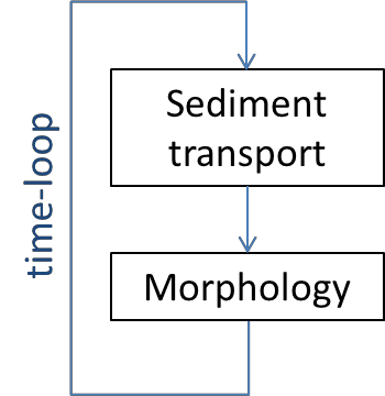
This should be done in two main steps (see also Figure 4).
The sediment transport rate \(q_t\) is first computed as a function of the local slope at each node (proportionality coefficient given in the Python script).
Hint
The local slope, defined as the gradient of the bed elevation (\(S = \partial \eta\)), can be computed using the numpy function gradient. When computing the slope, do these values make sense to you?
To compute the bed evolution per grid point, we need to calculate the difference between the sediment coming into the grid point and leaving the grid point. This is the amount of sediment that gets stored or eroded from that point, which changes the bed elevation. For bed evolution, the sediment balance equation (also called Exner equation) is then used. You can see this as a derivative of the law of mass conservation. It can be written as:
that is to say, in a discretized form:
and therefore
In short, the gradient of sediment transport should be calculated and then used to update the bed elevation.
Note
A negative gradient of sediment transport implies that there is more sediment going out than going in, resulting in a lowering of the bed surface.
Note
This formulation of the Exner relation assumes that the volume of deposited or eroded sediment includes pore space between the particles. In a later exercise, where we calculate sediment mass flux without pores using the Engelund-Hansen or Meyer-Peter and Mueller functions, the Exner relation will be written including the pore space correction.
Important
Download the necessary files for this Chapter here.
EXERCISE 1 - A very simplified morphodynamic model#
Important
You are expected to hand in this code and answers to the questions in your separate document.
The script file very_simplified_model.py contains the structure of the model, and some commands to visualise the results.
Add in the initialisation part of the script the definition of the bed elevation vector \(\eta\) at \(t = 0\). The initial bed elevation decreases linearly with a slope \(S_0\). The bed elevation at \(x = L\) (downstream boundary) should be zero. Data: \(L = 10\) m and \(S_0 = 0.1\) m/m.

Fig. 4 A very simple morphodynamic model system without flow#
Complete the time-loop using the explanations and equations given above in 3.1 A very simplified morphodynamic model.
Run the model and analyse the results. Report about your findings and explain what happens.
Let’s now modify the upstream boundary condition. We set the sediment transport rate \(q_t\) to zero at the upstream boundary (node 1, \(x = 0\)). This means that there is no incoming sediment flux in our model. Run the code. Interpret and report about the results.
Create a vector which contains the time-evolution of the bed elevation at the first node. This vector should be filled element-by-element during the time loop. Plot this vector as a function of time. What kind of evolution do you obtain? Despite the simplicity of this model, this behaviour is a fair representation of many morphological developments in nature.
Important
End of Exercise 1.
Please add this script and the document with answers to the open questions to the folder that you will zip and send to us.
3.2. Flow computation: backwater equations#
The model in the previous section was rather simplified: you already know that sediment transport depends on flow conditions, and the flow depends on discharge, channel dimensions, channel slope and bed roughness. To model the river in a physically more correct way, that is also more easily compared to reality, we must therefore compute the flow in the channel at each iteration and then use this updated flow to compute the sediment transport and the bed evolution. In this section, we present the backwater equations, which will be used in the next section to compute the flow in a more complex morphodynamic model.
More precisely, the flow in the channel will be computed using the backwater formulation for steady, gradually varied flow for subcritical flow typical of lowland rivers. Because the flow is assumed to be steady (imagine a morphologically relevant discharge of a previous exercise), we prescribe constant upstream water discharge per unit width \(q_w\) and impose a water surface elevation \(\xi_d\) at the downstream boundary (for example, the sea). Let \(H\) denote depth, \(\xi\) the water surface elevation, \(\eta\) the bed elevation, so that \(\xi = H + \eta\), \(k_c\) the total roughness height and \(S\) the bed slope.
The backwater equation is written as:
where \(F_r\) the Froude number defined as:
with \(U = \frac{q_{w}}{H}\). The bed friction coefficient \(C_f\) is assumed to follow a Manning-Strickler resistance relation, which is empirically similar to the White-Colebrook relation used earlier:
with \(\alpha_r = 8.1\).
Note
Here we use a notation taken from Prof. Gary Parker, whose teaching has made this kind of modelling accessible to students with diverse backgrounds. See his free online E-book here: http://hydrolab.illinois.edu/people/parkerg/morphodynamics_e-book.htm.
Frustrating fact: as usual in this world of many equations, notations and choices vary. For example, Parker prefers the Manning-Strickler relation because it is a power function, which is more easy to manipulate mathematically than the logarithmic relations used earlier, which are physically more correct.
How to solve the backwater equation:#
The backwater equation is first re-written in a discretized form (\(H_i\) being the water depth at the \(i\)th node):
where \(F_{back}(H)\) is a function defined as:
Adding a discretized form for \(S\) and inserting Eqs. (16) and (17) into Eq. (19) yields:
Rearranging equation Eq. (18), we get:
In practice, the resolution is performed in two steps in the code using a predictor-corrector scheme:
A first estimation of the water depth \(H_{temp,i}\) is computed (predictor step):
\(H_{pred,i}\) is then used to obtain a more precise prediction of the water depth (corrector step):
The water depth \(H_i\) at the node \(i\) can be therefore computed using the water depth \(H_{i + 1}\) one node downstream. The equations are solved starting from the downstream boundary (node \(N_x + 1\)), where the water depth \(H(N_x + 1)\) is known:
with \(\xi_d\) the water surface elevation imposed by the user.
Note
Think for a moment: since backwater effects work from downstream to upstream in subcritical flow, it makes sense to start calculating the water surface elevation from the downstream boundary in upstream direction.
This is one of the simplest numerical solutions that provides reasonably stable numerical solutions. You can easily make this model explode by making the timesteps too large or the length steps too small, so that it starts oscillating the water surface elevation somewhere between plus and minus infinity. More complicated numerical solutions exist and code for this can be found online with information for what sort of stability and accuracy these schemes were designed.
EXERCISE 2 - Flow computation using backwater equations#
Important
You are expected to hand in this code and answers to the questions in your separate document.
In this exercise you will need the scripts backwater_equation.py and functions.py.
Identify the different steps in the computation of the water depth \(H\). Why is the loop starting at \(N_x + 1\) and not \(0\) as usual?
Run the script and analyse the output.
The normal water depth \(H_n\) and critical water depth \(H_c\) are computed at the beginning of the script. Explain what these depths represent. Add to the figure two lines corresponding to \(H = H_c\) and \(H = H_n\). Make sure that these depths are plotted above the bed elevation. Modify the legend.
Run the code for different values of \(\xi_d\). Different behaviours can be observed depending on this value. Make a representative figure for each type of observed behaviour (to add to your separate document) and comment on your findings. Discuss in particular what is happening for values less than critical depth.
For insight into the numerics, now calculate a second vector \(H2\) which contains the water depth values obtained without using the corrector step. Plot the results with and without the use of a corrector in one figure and compare them. This comparison should be performed for a fine spatial grid (the one initially given for instance) and a very large one. Do you understand better why schemes such as the predictor-corrector are used?
Important
End of Exercise 2.
Please add this script and the document with answers to the open questions to the folder that you will zip and send to us.
3.3 Morphodynamic model with flow computation#
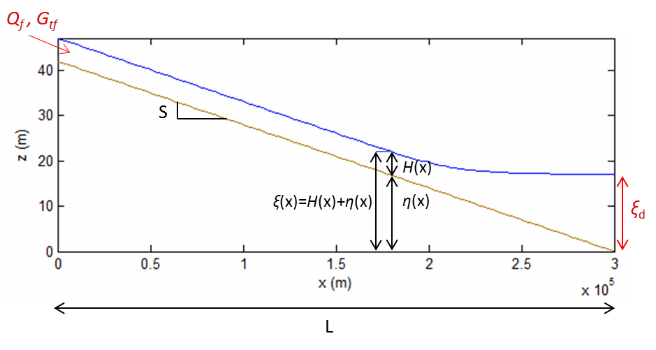
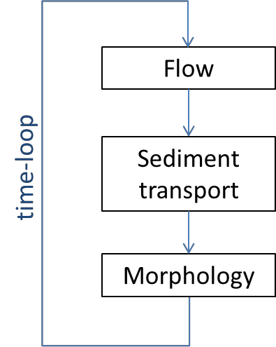
The model studied in this section is based on the same formulation as the spreadsheet RTe-bookAgDegBW.xls from the Gary Parker e-book. It allows you to compute the variations of the bed level \(\eta\) in space and time for different upstream and downstream conditions (variables in red in Figure 5). The model contains 3 steps, summarized in Figure 6.
The first part computes the water depth and flow velocity based on the backwater equations presented in 3.2. Flow computation: backwater equations.
The sediment transport is then computed using the flow characteristics determined in the previous step.
Finally, Exner equations are used to calculate the bed elevation from the sediment transport fluxes.
Note
This model is simple and fast, and assumes a constant and morphologically relevant flow discharge. This means that this model is useful for computations of long-term, large-scale morphological change in response to forcings such as changing average discharge, sea level and tectonics. Other kinds of models are needed to compute effects of individual floods, small-scale interference such as local bank protection, and bars and bends. Understanding what a model is not able to do also is important knowledge.
EXERCISE 3 - Implementing Parker’s morphodynamic model#
Important
You are expected to hand in this code and answers to the questions in your separate document.
For this exercise you will need the scripts model.py and functions.py.
A detailed description of the model is given in Chapter 20 of the Gary Parker e-book. Open this document (downloadable as a word document) and use it to identify the different parts of the script model.py. Look through the different functions called in this script and try understand what is going on.
Run the script. Why does the bed not change?
Use the word document with the model description to implement the sediment transport block in the model. Change the definition of \(q_t\) and remove the command
qt_u = 0, which set the sediment transport at the upstream boundary to zero. Calculate the shear stress from the flow velocity and friction; not from the depth slope product (see the model description).Run the script again, analyse the output. Where is sediment deposited and why?
What is happening when you enforce an instantaneous rise of sea water level (downstream boundary) while keeping the sediment input constant? Explain why this happens in terms of the underlying physics of backwater effects, sediment transport and sediment volume continuity (the Exner equation).
What is happening if you decrease the sediment input (upstream boundary)? Why?
In the Rhine, both happened at the same time. What happens then?
This is where the fun starts. Play with the model!
Note
Your model might produce incorrect results for some values of grid size and time step. More precisely, if the hump on the bed migrates more than one grid step \(dx\) during one time step \(dt\), the model becomes unstable. This gives the following stability condition (also known as the Courant-Friedrichs-Lewy (CFL) condition):
where \(C\) is the characteristic celerity of a disturbance in bed level. In practice, it means that if you significantly increase \(dt\) (to decrease your computation time for instance), you may have to increase \(dx\) to keep the model stable. Keep in mind that increasing \(dx\) decreases the spatial resolution of your model.
Important
End of Exercise 3.
Please add this script and the document with answers to the open questions to the folder that you will zip and send to us.

Fig. 5 Initial condition and variable definitions#

Fig. 6 The morphodynamic model system from Gary Parker#
PRODUCTS TO HAND IN#
The following exercises have to be handed in for the practical of Chapter 3:
Important
We expect the scripts and the separate word or PDF document in one zip file named YourSurname_GEO4-4436_Chapter3. Also include to your zip file all the separate files that you have imported in your scripts. Moreover, each script should be well labelled and contain the answers to questions should be provided in the word file. Please note that only the relevant information should be displayed when running the scripts, so do not print every variable.
Important
The final grade for the exercises of Chapter 3 is determined as follows:
Does the program run? (20%)
Does the program do what the assignment asked it and are the comments clear? (20%)
Are the answers to the questions correct? (20%)
Do the answers to the questions show insight of models and implications on reality? (20%)
Does the program produce clean figures? (20%)
Each of the sub-grades is graded between 0 (poor) and 5 (well done). The final grade for the exercises of Chapter 3 will make up 5% of the final grade of the course.