Chapter 1 - Starting programming with Python

Chapter 1 - Starting programming with Python#

Important

NOTES ABOUT CHAPTER 1

The exercises in this chapter will be graded on the following criteria: (1) Does the program run? (2) Can we understand it (= properly commented)? (3) Does it do the right thing as specified in assignment? See the end of this chapter for the full rubric.
There are 4 exercises that you must hand in, that increase in difficulty and time required for completion. Try to schedule your workload accordingly.
Please note, for this exercise you must submit the scripts (with appropriate comments) as a .zip file, which will be used to determine your grade.
The deadline for this Chapter is at 9:00 before the start of next practical.

1.1 Getting started#

While there are some good Python books, the best material for learning most things Python is online, thanks to the large Python community.

For this course, we write our Python files using an IDE (Integrated Development Environment), which is a software application that provides for user-friendly programming. There are many free IDEs to write code in Python. Here we use Spyder.

Note

Make sure you have completed the Software installation in order to be able to run Spyder in the course environment.

1.1.1 Overview on Spyder#

The Spyder interface is split into multiple parts:

Editor – this is where you will write your code.
Console & log – when you run your code, the outputs and errors will be displayed here. In the console you can also give commands, e.g. to get instant output or for testing lines of your code.
Multipurpose Window – this is where all the files, variables and plots in your workspace are listed and displayed.

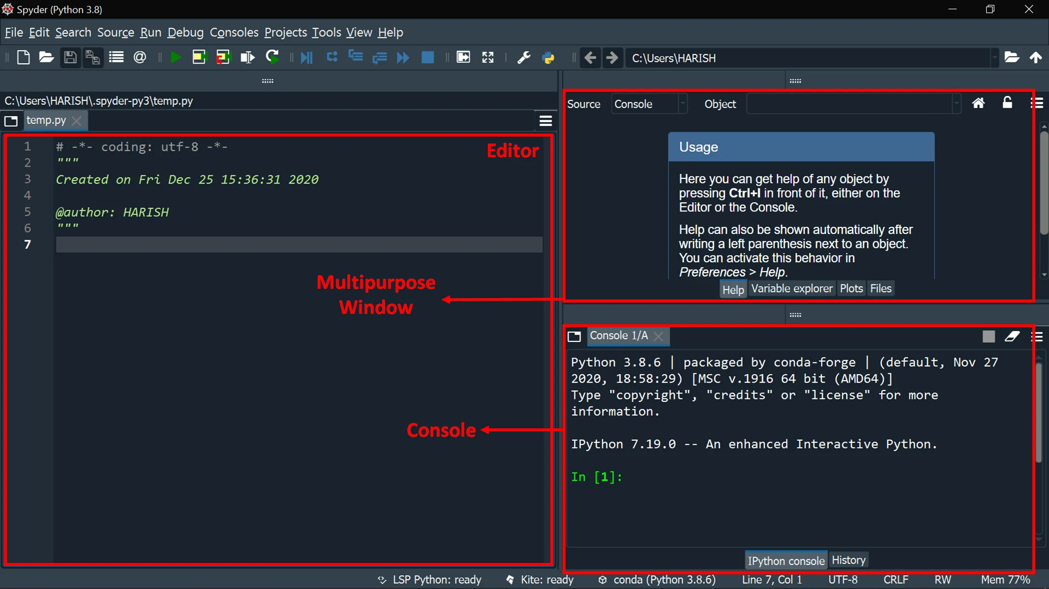
../_images/image1.png — Fig. 1 Setup of Spyder text editor. Source: Harish Maddukuri#

1.1.2 Creating your own workspace (directory)#

Python scripts are generally created and saved into Projects. These projects are located in a workspace/directory. The current workspace or directory is shown in the taskbar.

We advise you start every new practical by creating a new Project. To do that:

Projects $\rarr$ New Project
Give the project a name, e.g. Practical1
Enter the location where you would like to save the project

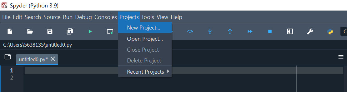
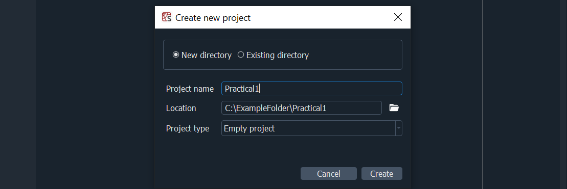
../_images/image3.png — Fig. 2 Creating a new Spyder project#

Any files that you create will now all be found in your project at the location you specified. In this project we can now have multiple scripts in the form of .py files. You can also click on the following icons:

to create a new .py file
to open an existing .py file
to save the currently displayed .py file
to save all open .py files

Now create a new project and a new file called Practical1.py. This is the file you will be working in today.

Note

For the coming exercises, you need to create different .py files. Don’t code the exercises in the Practical1 file.

1.1.3 Python basics#

Variables and operations#

In this section we will perform some introductory exercises of Python. We will do the following exercises in the Console. So leave your Editor empty for now.

Type in the console: print("Hello, World!") and then press enter.

You can see that the output prints the text (=string) you just wrote between the quotation marks.

Tip

Definition A string (‘str’) is an object that Python displays as-is and does not interpret, such as text that is intended for the human user. You can create a string by putting the text in single (' ') or double (" ") quotation marks.

For example, in the code print("Hello, World!"), the sequence Hello, World! is a string. The word print is a function (we will learn about these later), a type of instruction to the computer. If we were to write "print" instead, Python would no longer interpret this as an instruction, and would not pring the subsequent string to the console.

To verify whether this is indeed a string, run: type("Hello, World!").

You just asked the Spyder console to directly display information. Python will immediately forget this information after displaying it. For Python to remember information for future use, we need to store it in a variable.

For instance, declare variable a by running: a = 2.5.

With this command, we declare a new variable a and assigned the value 2.5 to it.

Tip

Definition A variable is a container for storing information. It has a name, such as a, and a value, such as 2.5. The value of a variable may be a number, a string, or an entire collection of such objects. Pretty much anything can be stored in a variable.

Assigning a value to a new variable is known in programmer-speak as declaring that variable.

Important

Assigning a new value to an existing variable will delete the old value of that variable. For example, if we run: [1]: x = 5 [2]: x = "Hello, World!" only the value “Hello, World!” will be stored in the variable x.

Now type in the console: b = 3 * a ** 2 and press enter.

We declared a new variable, b, equal to $3a^2$.

To see the value of b, run print(b) or just b in your console.

Important

Printing to the console As you can see above, when working in the console it is enough to type a command or variable name, and its result or value will be printed (shown) on screen.

In the next section, we will start working in .py files (a.k.a. code files or scripts). With these, only objects or outputs that are explicitly printed using the print function will appear on screen. Everything else will remind behind the scenes, as it were.

You can also navigate to the Variable Explorer. This provides the name, type, size, and value of the variables that are currently stored in the Spyder application.

The basic Python operations and their symbols are presented in Table 1. The most important data types for this course are listed in Table 2.

Table 1 Basic Python operations and associated symbols#
Operation	Symbol
Addition	+
Subtraction	-
Multiplication	*
Division	/
Exponentiation	**

Table 2 Most important data types in Python#
Type	Description	Example
`str`	String; text	`"Hello, World!"`
`int`	Integer; numeric	`2`
`float`	Float; numeric	`2.5`
`bool`	Boolean	`True` or `False`

Important

Reserved words and built-in functions Some terms in Python have a specific pre-defined meaning. In Spyder, these will appear in yellow or purple. If you type a name for a new variable and it changes colour, STOP! Giving this name to a variable will delete its built-in functionallity and could cause your code to behave “unexpectedly” (this is a programming euphamism for “disasterously”). Chose a different name for your code, e.g. my_list instead of the function name list. Examples of reserved words include the names of data types listed in Table 2, as well as the booleans True and False (but not true or false).

Initial lines of a Python script#

Now we start working in the Editor. A new .py file in Spyder will automatically show some initial information, e.g.:

# -*- coding: utf-8 -*-
"""
Created on Tue Apr  4 12:00:00 2023

@author: userName
"""

For EVERY future Python script you will make, it is important to add information that tells any viewer what this script is about. This is handy both for you and for others who want to see your script at a later moment. For instance, you could add to your Practical1 file:

"""
This script calculates the "Python Basics" exercises of Practical 1
for the course River and Delta Systems (GEO4-4436) at Utrecht University.

Created on Tue Apr  4 12:00:00 2023

@author: userName
"""

Note

The # -*- coding: utf-8 -*- is a remnant of an older Python version. You can ignore and delete this.

Running a Python script or specific lines#

Add two new lines to your script where you declare the same variables a and b as you did earlier above.
Add print(b) in a new line.
Now run your script by clicking:

What do you observe in your console and variable explorer?

Select all lines of code in your Editor.
Press F9.
Now do the same with just selecting the line which states print(b).

Note

Note: there is a difference between RUNNING the file (using the green play button) and executing it in the console. Execution in the console is much slower than simply running the file, works great for validating whether specific lines in your code actually work.

Clearing the console and variable explorer#

Clear the console using the clear button
Now type in the console: c = a * 30 and press Enter

We are declaring a new variable $c$, as a function of variable $a$, but you just deleted $a$. The command cannot be executed, because $a$ is not stored in Python’s memory anymore. An error message appears in the console.

Python functions#

You might imagine that doing lots of complicated calculations and working on large datasets may result in extremely long and complicated scripts. To counter this, you can break up programming tasks into separate functions, which include the following advantages:

Simplicity: functions typically focus on a small task rather than an entire problem.
Maintainability: if functions have a high degree of independence from each other, updating one such function will have limited impact on other functions.
Reusability: functions can easily be reused in a script, limiting duplication of code.

Run in your console:

from numpy import pi
from numpy import cos

You just imported two object – one is the constant pi and the other is a function that calculates the cosine of a value. Run: cos(pi). Now clear the console and run cos(pi) again. Clearing the console also deletes all imported objects!

Now, what exactly is numpy?

Python packages#

The advantage of Python is that it is free and open-source, where any user can write code and functions and share them online for anyone to use. This isn’t limited to individual users, but also applies to big software development teams. If such a team has developed a large set of functions, they typically store them in a library or package. One such important package is NumPy, which provides numerous mathematical functions and is widely applied in scientific calculations.

Instead of importing separate functions (e.g. numpy.cos), you can also import the entire package. Add to your Editor and run:
```
import numpy as np
```
Note

The as np tells your program that wherever a command starts with np. it needs to look it up in the NumPy library.

Note

For any package or function that you want to import, it is important to do this at the beginning of your Python script, before using them!

If you import a package but don’t use it, an orange triangle will appear to the left of the import command in the Spyder editor.
Run your script and you can use all of the functions available in the NumPy library. Run in your console: np.cos(np.pi) and then cos(pi). Do you understand the difference here?
Now test some of the other frequently-used mathematical functions of NumPy, given in Table 3.

Table 3 Several important mathematical functions in *NumPy*.#
Functions	Description
`np.sin()`, `np.cos()`, `np.tan()`	sine, cosine and tangent (arguments in radians)
`np.arcsin()`, `np.arccos()`, `np.arctan()`	inverse sine, cosine and tangent
`np.abs()`	absolute value
`np.sqrt()`	square root
`np.round()`	round towards the nearest integer
`np.ceil()`, `np.floor()`	round towards plus (`ceil`) or minus (`floor`) infinity
`np.log()`, `np.log10()`	natural logarithm, logarithm base 10
`np.exp()`	exponential

Important

All of these mathematical functions have their own documentation at the official NumPy web page, or on many of the other Python-related web pages. A very important step of debugging is always to ask a search engine! Also see the the debug manual on Brightspace. Note, however, that asking an Artificial Intelligence to write your code will not help your learning (and may count as plagiarism, and has an enormous CO₂ footprint).

If you want to see all the attributes of a function or package, run for instance help(np) or help(np.cos).

Aside from NumPy, there are countless other free and open source packages that constitute the vibrant community of Python. As you will find out later, other important packages in this course are:

pandas, which is handy for data analysis and manipulation.
matplotlib, which is used for data visualisation.

Note

A Python function is specific to a single task. Packages can also include modules, which define multiple functions, classes, attributes etc.

1.2 Working with .py files#

A .py file is a program file or script written in Python. It is a succession of Python commands which can be written and edited using a text editor and then is run using the Python interpreter - this is the behind-the-scenes part of Python, which translates our code into something the computer can understand directly. A Python IDE such as Spyder contains a text editor (and other useful elements, as we’ve seen), and is capable of communicating directly with the interpreter. Using .py files allows you to organise and save different series of commands. Scripts can be edited, extended or corrected whenever you want and can be executed several times. Writing the commands into a script is necessary when you perform advanced data analysis, since it allows you to check/improve your methodology, but also to be sure you perform the exact same data processing for several datasets, for instance.

Important

Good code includes comments to explain to anyone reading what different parts of it do - most importantly to Future You, who will be staring at the script a month from now, wondering “wth was I trying to do here?” Comments in Python start with a #, which tells the interpreter to skip the rest of the line and move on to the next one. In Spyder, comments will appear in a different colour (grey by default).

When a script is executed, Python executes the commands in the order they are written. It is therefore important to consider in which order you want to execute your commands. Generally, scripts are structured as follows:

Docstring (documentation string) Describe the script in a few words (e.g. objective, date of creation, author of the script)
Package import Import all the necessary packages to perform operations (e.g. NumPy)
Initialization Declare the main variables and load your data
Calculations Execute the calculations
Output and visualisation Commands to display the results, plot graphics and save output

Copy-paste and execute the simple example below:

"""
This script provides an example of a "basic" structure of a .py file
for the course River and Delta Systems (GEO4-4436) at Utrecht University.

Created on Mon Apr  17 12:00:00 2023

@author: userName
"""

# Package import
import numpy as np
import matplotlib.pyplot as plt

# Initialization
a = np.array([0, 1, 2, 3, 4, 5])

# Calculations
b = a ** 2

# Output and visualisation
plt.plot(a, b)

Tip

Best practices for using Python are described in a series of “Python Enhancement Proposals” or PEPs. Most relevant to the beginning and even advanced Python user are PEP 8 - the style guide and PEP 20 - the Zen of Python (or run import this in your Spyder console).

EXERCISE 1 - Calculate river flow velocity and water depth#

Important

You are expected to hand in this code.

The aim is to calculate flow velocity and water depth in a river from known variables and parameters (use a web search to find out what the difference is between “variable” and “parameter”). The flow resistance parameter for this river is $C = 44$ m^1/2/s, the discharge $Q = 2500$ m³/s, the channel width $W = 500$ m and the channel gradient $S = 1.6 × 10^{−4}$ m/m. $Q$ is defined as:

(1)#\[\begin{split} Q = h u W \\ \end{split}\]

where $h$ is water depth in m and $u$ is flow velocity in m/s averaged over the depth and width of the channel. $u$ is related to $h$ following the Chezy equation:

(2)#\[\begin{split} u = C\sqrt{h S}\\ \end{split}\]

See Kleinhans, 2005 for a brief overview how the Chezy relation is equivalent to the Darcy-Weisbach relation and the Manning relation, which you might be more familiar with.

The commands should be written in a file called Exercise1.py, saved in your current directory. The script should print the results.

Do not forget to comment the file and give meaningful names to the variables.

Hint

$S = 1.6 × 10^{−4}$ can be written in Python as: 1.6e-4.

Important

End of Exercise 1.

Please add this script to the folder that you will zip and send to us.

1.3 Data structures#

A data structure is the fundamental form that Python uses to store and manipulate data. It allows for efficient calculations and analysis over entire datasets. There are multiple types of data structures. In this course we will discuss lists, arrays and DataFrames.

A list is simply a one-dimensional series of elements (e.g. numbers, strings, other lists, or a combination thereof). You can a list create using square brackets [] or the list() function, e.g. my_list = [1, 2, 3, 4, 5] and my_list = list((1, 2, 3, 4, 5)) will produce the same result.
An array is similar to a list, but it can have any number of dimensions. An array contains data of all the same type (e.g. all integers or all strings). Python has a built in function array(), but you will usually want to use NumPy to manipulate your array, therefore it would be better to use the NumPy function np.array().
A DataFrame is a table of different elements organized in rows and columns which CAN be of different datatypes (although each column can only have one data type). We use the pandas library to work with DataFrames.

Different data types that can be stored in lists, arrays and DataFrames are provided in Table 2.

In this section we will learn how to create lists, arrays and dataframes, extract the relevant information from one of them, and perform calculations with them.

Tip

There are more data sctructures you should be aware of, as they are in highly common use in Python:

A tuple is similar to a list, but it cannot be changed once it has been created, while a list can. A tuple can be created using parens: my_tuple = (1, 2, 3) or the tuple() function: `my_tuple = tuple([1, 2, 3]).
A dictionary, or dict stores data in pars of keys and values (think of the keys as labels or names), e.g. my_dict = {"spam": 50, "egg": 46}. Follow the link for more details. A common way to create a DataFrame is from data stored in a dict.

1.3.1 Creating lists, arrays and DataFrames#

Clear your variables and run in your console: my_list = [1, 2, 5, 10]. Check the Variable Explorer to see the type of data structure that is produced.
Now run in your console: my_list2 = [[1, 2, 5, 10], [3, 4, -2, 7]]. Now compare my_list and my_list2 in the Variable Explorer. Do you understand the difference in size?

Hint

By double clicking on a variable in the variable explorer, you can see more information.

my_list and my_list2 are data structures of the type list. A list is a basic Python structure included in the core Python modules. It therefore does not require a package to be imported.

Now import NumPy again as np.
Run: my_array = np.array(my_list2). What kind of variable do you obtain and how is different from my_list2?

my_array is of type array, which is a data structure type of the NumPy package.

Now run: import pandas as pd and df = pd.DataFrame(my_list2). What is the difference between my_list2, my_array and df?

Note

Similar to importing NumPy as np, it is very common to import pandas as pd.

df is of type DataFrame, which is a data structure type of the pandas package.

Now run: my_array2 = np.array(df) and df2 = pd.DataFrame(my_array). Are there differences between my_array and my_array2 or df and df2?

NumPy arrays can be easily transformed into pandas DataFrames and vice versa.

Important

Some functions, classes or attributes require a specific type of data structure (e.g. array or DataFrame). Therefore, you should always consider whether your variable is stored in the proper data structure!

The advantage of package-built data structures is that they have their own built-in attributes. Attributes are accessed by appending them with a . after the object or variable name.

Run the following code:

df.size

df.shape

my_array.size

my_array.shape

As you can see, there are overlapping attributes between NumPy arrays and pandas DataFrames. For any type of data structure, you can usually find the attributes online in the official documentation of the specific data structure (e.g. pandas DataFrame).

Have a closer look at the attributes listed in the DataFrame documentation. Run the following codes:

len(df.index)

len(df.columns)

Do you understand what the above lines display and what the funcion len() does?

Instead of defining all the specific elements, as you did for my_list and my_list2, you can also define an array of a number of elements following an interval. You can do this using the NumPy function np.arange:

Run the following codes:

my_array3 = np.arange(1, 6, 1)

my_array4 = np.arange(1, 6, 2)

my_array5 = np.arange(12, 0, -3)

my_array6 = np.arange(12, 0, 3)

Compare the outcomes. Do yo understand how the np.arange function works?

The np.arange function requires as input “(begin, end, interval)”. If no interval is specified, the default interval is 1. So np.arange(1, 6) will return the same as np.arange(1, 6, 1).

Note

The end number is not included in the output array.

Thus np.arange(1, 6, 1) returns [1 2 3 4 5] and NOT [1 2 3 4 5 6].

1.3.2 Concatenation, vstack and hstack#

Sometimes it can be useful to combine several related arrays or lists into one unique array and join them together. This can be done using the NumPy function np.concatenate.

Clear your variables and import NumPy. Run the following codes:

array_a = np.arange(1, 3)

array_b = np.arange(4, 6)

array_c = np.concatenate((array_a, array_b))

Inspect how arrays array_a and array_b are joined together into array_c.

Note

Notice that we used double parens (parentheses, ()) for np.concatenate. This is because the function requires that we give it a sequence of arrays or lists to concatenate. In this example, we used a sequence of type tuple (denoted by the surrounding ()), but we could also have used a list, like this: np.concatenate([array_a, array_b]).

The default is to concatenate arrays in the same dimension (also referred to as horizontally).

Note

The above arrays are 1-dimensional (i.e. their size has only one direction, for example (2,) and not (2,1)). Double-clicking a 1-dimensional vector in the variable explorer provides a default vertical display. Don’t mistake this for a 2-dimenstional display of several rows and one column (e.g. (2,1))!

Now run:

array_d = np.vstack((array_a, array_b))

array_e = np.hstack((array_a, array_b))

Compare the outcomes.

NumPy vstack is used to vertically concatenate arrays, whereas hstack is used for horizontal or 1-dimensional concatenation (for the situation above, array_c and array_e yield the same concatenation output).

Note

concatenate, hstack and vstack can be used to combine strings, and lists or arrays of floats and integers (Table 2). To vertically stack two lists they must have the same dimensions!

1.3.3 Manipulating data structures using index numbers#

Elements in data structures are usually identified by their position (row and column numbers), also called their index number. Table 4 shows how the different elements of a 3 × 6 matrix can be identified using their index numbers.

Table 4 Subscripts of 3 × 6 matrix#
[0,0]	[0,1]	[0,2]	[0,3]	[0,4]	[0,5]
[1,0]	[1,1]	[1,2]	[1,3]	[1,4]	[1,5]
[2,0]	[2,1]	[2,2]	[2,3]	[2,4]	[2,5]

For a NumPy array you can identify an element by position as follows:

Clear your variables and import NumPy and pandas as np and pd, respectively. Run the following code:

my_list = [[1, 2, 5, 10], [3, 4, -2, 7]]

my_array = np.array(my_list)

val_a = my_array[1, 3]

Here val_a provides the element at position (1,3) of my_array.
Now try if this also works for a pandas DataFrame by running:

df = pd.DataFrame(my_list)

val_df = df[1, 3]

Here we refer to an earlier note on data structures.

To identify the element of a pandas DataFrame through a subscript, we use iloc (= index location):

Run:

val_df = df.iloc[1,3]

As iloc is an attribute of pandas DataFrames, it won’t work for a NumPy array. Try: val_a = my_array.iloc[1,3]
Write your own code that returns -2 for both my_array and df.

To replace an element with something else we use NumPy where or pandas replace.

Run the following code:

my_array = np.where(my_array == -2, 2, my_array)

df = df.replace(-2, 2)

Compare my_array and df with their previous outputs. Do you understand how the np.where function works?

Instead of single elements, you can also call entire rows and columns.

Run the following codes:

array_row = my_array[0, 0:4]

array_column = my_array[0:2, 2]

df_row = df.iloc[0, 0:4]

df_column = df.iloc[0:2, 2]

Examine the outputs.

Note

Instead of defining a row or column through its first and last index, you can also just use :, e.g. for the variables definede here, array_row = my_array[0, :] yields the same output as array_row = my_array[0, 0:4]. The same goes for df_column = df.iloc[:, 2] and df_column = df.iloc[0:2, 2].
Create two new vectors containing the second rows of my_array and df.
Replace all elements of the second columns of my_array and df with zeros.

1.4 Operations on NumPy arrays and pandas DataFrames#

1.4.1 Operations between a scalar and a matrix#

If you perform simple operations on a NumPy array with a scalar, that operation is applied to each element in the array.

For instance, inspect the outputs of the following commands:

2 * my_array

2 / my_array

2 + my_array

2 - my_array
Now try the same operations with pandas DataFrame df. Do these operations also work for Dataframes?

1.4.2 Operations between matrices#

Simple operations between arrays and DataFrames#

Addition or subtraction operations can only be applied to matrices of identical size. The resulting matrix is obtained by adding (subtracting) their corresponding elements. Example:

Define the following new matrix of same size as my_array and df and store it both as a NumPy array and as pandas DataFrame:

\[\begin{split} matrix = \begin{pmatrix} 3 & 8 & 0 & 160\\ 13 & 42 & 21 & 17 \end{pmatrix} \end{split}\]
Now try operations of +, -, *, / and ** between my_array, df and matrix. Also try operations between arrays and DataFrames. Inspect the outputs.

Multiplication of two matrices#

Matrix multiplication according to linear algebra follows different rules.

Define two new arrays array_b and array_c:

\[\begin{split} array_b = \begin{pmatrix} 1 & 0 & 2\\ 5 & 10 & 7 \end{pmatrix} \quad \textrm{and} \quad array_c = \begin{pmatrix} 1 & 3\\ 4 & 1\\ 2 & 2 \end{pmatrix} \end{split}\]
To execute a matrix multiplication, you use np.matmul, run:

array_d = np.matmul(array_b, array_c)

This will calculate the matrix product of array_b and array_c as follows:

\[\begin{split} array_d(i,j) = \sum_{k=1}^{n} array_b(i,k) \ast array_c(k,j) = \begin{pmatrix} 1 \ast 1 + 0 \ast 4 + 2 \ast 2 & 1 \ast 3 + 0 \ast 1 + 2 \ast 2\\ 5 \ast 1 + 10 \ast 4 + 7 \ast 2 & 5 \ast 3 + 10 \ast 1 + 7 \ast 2 \end{pmatrix} = \begin{pmatrix} 5 & 7\\ 59 & 39 \end{pmatrix} \end{split}\]

1.5 Python built-in functions for arrays and DataFrames#

1.5.1 Examples of elemantary functions#

NumPy functions can generally be used on all sorts of matrices (including NumPy arrays and pandas DataFrames). However, both NumPy arrays and pandas DataFrames have many of these functions as built-in methods (the technical term for a function that is written into the definition of a data structure or other programmatic type). A method of a NumPy array is usually just another way of writing the equivalent NumPy function. However, the equivalent method for a non-NumPy matrix (e.g., a DataFrame) will often be better adapted to use with that specific data structure.

For example, np.mean() returns the mean value of a matrix. When applied to a NumPy array, np.mean(my_array) returns the same result as the array’s built-in method my_array.mean(). Applying this to a DataFrame containing the same values np.mean(df) will, again, return the same result. However, the DataFrame’s built-in method df.mean() will return a different result. Try it for yourself and see if you understand what it does. Check the documentation to learn the different ways you can apply this method, including how to get the same result as with np.mean(df).

Note that NumPy functions that manipulate values in a matrix can also be applied to an individual value.

We are now going to look at several additional examples of functions for both arrays and DataFrames. For a complete list, go to the official documentation of NumPy arrays and pandas DataFrames. If you’re looking for something specific, it’s always a good idea to conduct an online search for the data structure you are using.

It is possible to round the value of floats and matrices using np.round or pandas.DataFrame.round. Run the following and inspect the outcomes to see if you understand what happens:

np.round(1.555)

np.round(1.555, 2)

np.round(my_array / 3)

(my_array / 3).round()

np.round(df / 3)

(df / 3).round

The last example could also be written as:
```
df = df / 3
df.round()
```
To transpose a matrix, you change the rows of the matrix into columns, and vice versa using np.transpose. As a consequence, a matrix of size n × m will turn into a matrix of size m × n containing the same elements organised in a different way.

np.transpose(my_array)

np.transpose(df)

df.transpose()
To create new arrays, you are not required to write down every element, such as you did earlier by defining my_list. Run the following and inspect the outcomes:

np.zeros((3, 5))

np.ones((5, 3))

np.full((3, 5), 2)

np.full((3, 5), np.nan)
With the help of functions previously introduced, create a matrix of size 20 x 30 containing only floats that represent $5 / 3$ to six decimal places. Try to do this in only one line of code!

1.5.2 Data analysis#

The main functions and methods available to perform (statistical) data analysis on arrays are summarized in Table 5. Some examples of the use of these functions are given below.

Define the following vector as an array:

vect_A = np.array([6, 2, 5, 7])
Run the following commands and inspect the outputs:

vect_A.mean()

vect_A.median()

vect_A.sum()

vect_A.max()

vect_A.min()
In some practical cases, it is important to know when a maximum (or minimum) value has been reached, that is to say, what is the position of the largest value in the original array. To return the index/location of the max or minimum value use np.argmax or np.argmin, respectively. The equivalent pandas methods are df.idxmax and df.idxmin. Inspect the following:

vect_A.argmax()

vect_A.argmin()
Now run:

s = np.sort(vect_A)

Compare s and vect_A.

Table 5 Some important functions and methods for statistical data analysis on matrices#
NumPy	pandas	Description
array.max	df.max	Maximum value
array.min	df.min	Minimum value
array.median	df.median	Median value
array.mean	df.mean	Average/mean value
array.std	df.std	Standard deviation
array.var	df.var	Variance
np.percentile	df.quantile	Percentile values
array.sum	df.sum	Sum of the elements
np.sort	df.sort_values	Arrange the elements in ascending order (pandas: sort the DataFrame following the order of a specific column)

EXERCISE 2 - Array calculations#

Important

You are expected to hand in this code.

Make a new file called Exercise2.py in your work directory. The script should print the results of all assignments.

Create the following NumPy array my_array:

\[\begin{split} my\_array = \begin{pmatrix} 16 & 3 & 2 & 13\\ 5 & 10 & 11 & 8\\ 9 & 6 & 7 & 12\\ 4 & 15 & 14 & 1 \end{pmatrix} \end{split}\]

Create an array array_1 containing the first row of my_array.
Create a scalar, sum_a1, equal to the sum of the elements of array_1.
Create a vector sum_rows, where each element contains the sum of the elements of one of the rows of my_array. The first element of this vector should be equal to:

\[ sum\_rows[0] = \sum_{k=0}^{4} array_1[0,k] \]

Try to do this in one line!
Create a vector sum_columns, containing the sum of the columns of my_array.
What do you notice when comparing sum_rows and sum_columns?

Include answers to open questions as strings and print them to the console.

Important

End of Exercise 2.

Please add this script to the folder that you will zip and send to us.

1.6 Visualising data#

How to make a simple 2D-plot: example

Add all the following lines of code to the file Practical1.py in your Editor, not your console!

Clear your variables, import NumPy and create the following arrays in your file:

x = np.arange(- np.pi, np.pi, 0.5)

y = np.sin(x)

y2 = np.cos(x)
Now we will use the package matplotlib to create a figure. Add to the beginning of your file:

import matplotlib.pyplot as plt
Add to your file the following lines of code:

plt.figure(1)

plt.plot(x, y)

plt.show()

Note

You have to include the plt.figure(1) because you have to give unique numbers to your separate figures in your script.

Select all the lines you have in your file and press F9. Inspect what happens.
Now run in your console:

plt.plot(x, y2)

A new plot has replaced the previous one in the figure window. To display the second graph on top of the first one you have to edit your file as follows:
```
plt.figure(1)
plt.plot(x, y)
plt.plot(x, y2)
plt.show()
```
Run the following lines with F9.

Note

As is alwas the case in programming, the order of your lines of code is very important here!
Edit the second plotting line so it now reads

plt.plot(x, y2, color='r')

Run the lines. Do you understand what happened?
Title, labels on the x- and y-axes and legends can now be defined. Type the following commands (before plt.show()!) one by one and analyse their effects on the figure:

plt.title('Sine and cosine functions')

plt.xlabel('Radians')

plt.ylabel('Function value')

plt.legend(['sine', 'cosine'])
Matplotlib is the basic package for plotting your data, but there are also complementary packages that can be used to improve your figures further, such as seaborn. Include at the top of your script where you import your packages:

import seaborn as sns

sns.set()

Run the plotting lines again, do you see the difference?
To specify the limits of the x- and y-axes include for instance (before plt.show()!):

plt.xlim(- np.pi, np.pi)

plt.ylim(- 2, 2)

Run the plotting lines again. What has happened?
It is also possible to plot without specifying the x argument. Run:

plt.plot(y)

The elements are now plotted as a function of their position in the vector: y[0] at x = 0, y[1] at x = 1, etc.
Multiple plots can also be displayed in one figure. This can be done using the command subplot(a,b,c) where a, b and c are integers, and c is less than or equal to the product $a * b$. This command divides the figure in $a * b$ sub-figures, organized in $a$ rows and $b$ columns. To obtain 2 plots, one above the other, include and run following lines below your 1st figure:
```
plt.figure(2)
plt.subplot(2, 1, 1)
plt.plot(x, y)
plt.subplot(2, 1, 2)
plt.plot(x, y2, 'g')
plt.show()
```
Add labels and titles to your subplots of the second figure
To close a figure use:

plt.close()

Try this with and without the code plt.show().

Hint

You can easily disable a line of code by adding a #. This is known as commenting out inprogrammer speak.

Note

You can close the currently opened plot in your figure window by clicking:

You can close all plots in the figure window by clicking:
Numerous options are available to customize your plots, all lised in the official documentation of matplotlib. Some examples are given in Table 6. Try out the example in Table 6 in your own script.

Table 6 Some important matplotlib.pyplot functions for customizing your plots#
Syntax	Description
`plt.plot(x, y, color='r')`	Solid red line
`plt.plot(x, y, color='r', linestyle='--')`	Dashed red line
`plt.plot(x, y, color='r', linestyle='--', linewidth=2)`	Thick dashed red line
`plt.plot(x, y, color='g', marker='*')`	Green asterisks with line
`plt.plot(x, y, color='g', marker='*', linestyle='none')`	Green asterisks without line
`plt.plot(x, y, color='magenta', marker='s', linestyle='dashdot')`	Magenta squares with a dash-dot line

There are many colours available, using either letters, full names or colour codes. Search for matplotlib color or seaborn color to get an idea of what colours are available. The figure below also indicates a wide range of colour options. If you are using several lines it may be nice to use a Seaborn color palettes. An example of how to do this is as follows:

sns.set_palette("Spectral", 18)

In this case Spectral is the name of the palette and 18 is the number of lines you will use in your plot. Search for seaborn palettes to see what else is available.
Similarly, many marker and line styles are available. See the images below for the most common options.

Note

If you want to reset the Seaborn settings to original, run:

sns.reset_orig

If you want to switch off Seaborn, you can reset matplotlib within your script or through the console, by running:

import matplotblib as mpl
import importlib
Importlib.reload(mpl); importlib.reload(plt); importlib.reload(sns)

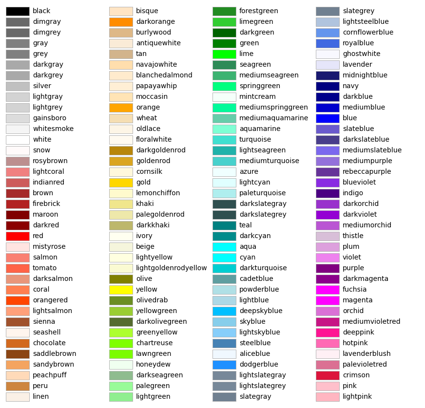
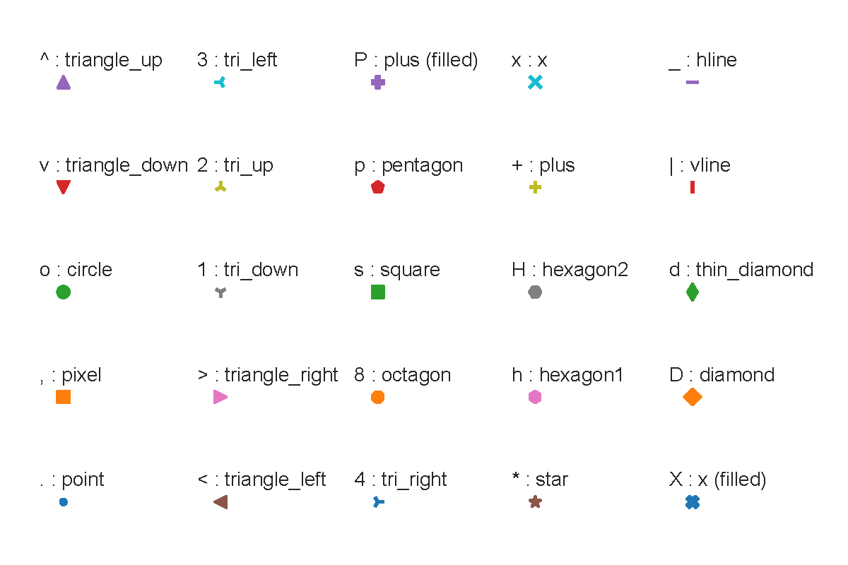
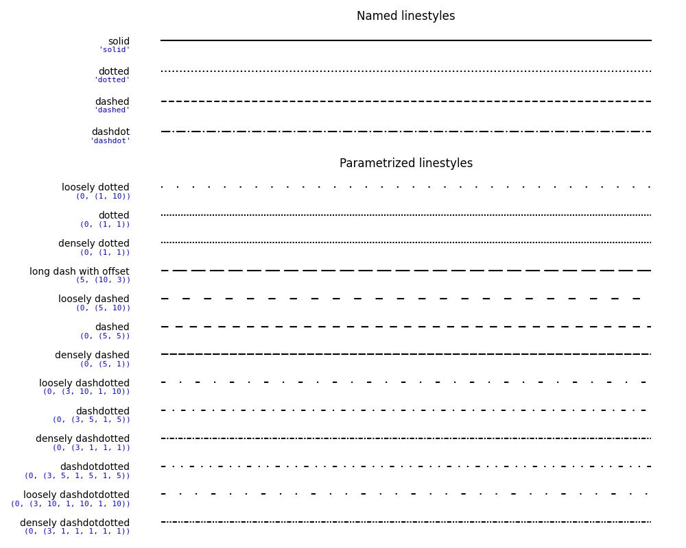
../_images/image15.png — Fig. 3 Specs for colors, markers and linestyles in matplotlib#

EXERCISE 3 - Visualisation of river sediment transport data#

Important

You are expected to hand in this code.

Important

Make sure to use plt.show() after every figure you are asked to make.

This exercise is based on the dataset contained in the file MPMtransportdata.xls. Meyer-Peter and Mueller (1948) (abbreviated MPM) graphically reported gravel transport data from their flume experiments and derived their famous empirical bedload transport predictor from this dataset. Wong and Parker (2006) recovered the original data and re-analysed it to find that the original fit by MPM was wrong. Here you will plot both the data in nondimensional form and plot a predicted transport using a sediment transport predictor. We assume that the density of the water $\rho=1000\ kg\ m^{-3}$ and Earth’s gravity acceleration $g=9.81\ m\ s^{-2}$ (the notation form $m\ s^{-2}$ is commonly used for units in technical documents, and is equivalent to $\frac{m}{s^2}$).

Make a new file called `Exercise3.py. Do not forget to clear your workspace and close the figures at the beginning of your script.
Download the file “MPMtransportdata.xls” from Brightspace or Teams and save it in your current working directory.
Important

For your code to be able to access a file, you must specify the filepath (or path, for short) to that file. This is the sequence of folders you would have to click through to get to the file, e.g., “C:\Users\username\Documents\myworkspace\MPMtransportdata.xls”. When you want to use this information in Python, you can type out the path as-is:
```
path = r"C:\Users\username\Documents\new_workspace\MPMtransportdata.xls"
```
Notice that a path in Python is always given as a string, and that in this example we have stored it in a variable called path, which we will later pass as an argument to the function that will access the file. The r is short for “raw” and tells Python not to apply additional meaning to anything in the string (for instance, the “\n” at the beginning of “\new_workspace” could also mean a line break).

The above filepath uses Windows syntax with back slashes (). Mac and Linux use forward slashes (/). When your code might be used on both system types (which IS LIKELY in this course!), you can avoid issues by specifying you filepath as follows:
```
import os # this goes at the BEGINNING of your script

path = os.path.join("path", "to", "file.extension") # replace strings with directory and file names in the correct order
```
This will combine the directory names into a single string, with directory and file names separated by “" or “/”, depending on the computer you are running the code on.

This can be simplified a lot by using relative paths, which tell Python where to go from the current working directory. So, if your data file is in the same directory as your Python script, you can simply write:
```
path = "MPMtransportdata.xls"
```
It is good practive to have a separate data sub-directory inside your project directory. Create a subdirectory called “data” in your project directory and put your data file in it. Now you can use the following relative path in your Python script
```
path = os.path.join("data", "MPMtransportdata.xls")
```
Remember to include the data sub-directory and its contents in your submission folder, or your script won’t run properly when the TAs test it!
You can now load the data using the following line:
```
mpm_data = pd.read_excel(path)
```
This reads data from the file into a pandas DataFrame. The function reads in ALL the information including the text headers, which is not convenient for calculations. Check the functions’ documentation for ways to exclude irrelevant data, so that you get a tidy DataFrame.

Hint

Try the skiprows parameter.
The data you will want to use are:
- the discharge $Q (m^3\ s^{-1})$,
- channel width $W (m)$,
- water depth $h (m)$,
- slope $S (m\ m^{-1})$,
- median grain size $D_{50} (m)$,
- the specific gravity of the sediment $s$ (which is density of sediment divided by density of water), and
- the sediment transport rate $q_s (m^2\ s^{-1})$ (or $m^3\ s^{-1}$ per $m$ width).
Make sure you understand the names of the columns.

Hint

Check the units of the dataset!

You can work with a specific column in the DataFrame using the syntax df[column name] (where column name is a string), e.g., mpm_data["DISCHARGE"] for the first column in the current dataset. You can also rename columns with df.rename. Most methods of a DataFrame also work on a single column (technically called a Series), e.g., mpm_data.mean() to get means for the whole DataFrame, or mpm_data["DISCHARGE"].mean() to get only the mean of this column.
In order to compute sediment transport, it is necessary to know the total bed shear stress $\tau$ (Pa). Calculate a new vector tau, using:

(3)#\[ \tau = \rho gh\sin{S} = \rho {u\ast}^2 \]

where $u\ast$ is the shear velocity ($m\ s^{-1}$), defined by the above relation. (Accept this for now… there is a complicated story behind it involving boundary layer theory.)

Note

It is possible that some of your columns will be read in with the wrong data type (such as numerical values being represented as strings instead of floats). If so, some mathematical functions will not work properly. If you run into problems, try searching for a method or function called astype and applying it to the relevant column in the DataFrame.
To compare datasets derived from different scales (e.g. field versus lab measurements), parameters are often made dimensionless. Shear stress $\tau$ can be nondimensionalized into the “Shields parameter” $\theta$, which is the ratio of the flow force driving sediment transport and gravitational force that demobilizes sediment. Calculate $\theta$ following:

(4)#\[ \theta = \frac{\tau} {\left( \rho_s - \rho \right) g D_{50}} \]

where $\rho_s = s \rho$ refers to the sediment density.
Sediment transport can be nondimensionalized with the “Einstein parameter” $\phi$. Calculate $\phi$ using:

(5)#\[ \phi = \frac {q_s} {(Rg)^{1/2}D^{3/2}_{50}} \]

wherein $R = (\rho_s-\rho)/\rho = (s-1)$ is the relative submerged density.

Hint

Make sure you use brackets to enclose fractions!
Plot the sediment transport rate $q_s$ (y-axis; this is the effect) as a function of the shear stress $\tau$ (x-axis; this is the cause). Plot the data as points in log-scales for both axes. To do that, the function plt.plot() can be replaced by plt.loglog(). Give an appropriate title to the plot, as well as labels to the x- and y-axes.

Note

When writing texts for figure titels or axis labels, writing sections of text between two $-signs will automatically make the text between these signs mathematical, e.g. $m^2$ becomes $m^2$. Similarly, $q_s$ will become $q_s$. To subscript or superscript more than one character, use the curly brackets {}, for example $D_{50}$ becomes $D_{50}$. To find out more about this type of formating, search for “Latex math”.

Note

To use Greek letters in your titels or axis labels, you can use $\greekletter$ , e.g. $\phi$ becomes $\phi$.

Hint

matplotlib.pyplot has a built-in interpretation for \t. To prevent this from affecting the texts of Greek letters such as $\tau$ or $\theta$ in your plots, assure by the dollar signs that your texts are interpreted as raw strings.
Plot in a new figure the data in a nondimensional form, i.e., the Einstein parameter $\phi$ (y-axis) as a function of the Shields parameter $\theta$ (x-axis). Give an appropriate title to the plot, as well as labels to the axes.
Compare the figures plotted at 7 and 8. What is the use of dimensionless variables?

Include answers to open questions as strings and print them to the console.
The MPM predictor of Meyer-Peter and Mueller (1948) was derived from flume experiments with bed load transport, meaning that it does not predict suspended load bed material transport. It is given as:

(6)#\[ \phi_b = 8 \left( \theta^/ - \theta_{cr} \right)^{1.5} \]

where the lower case “$b$” in $\phi_b$ refers to the Einstein parameter for bed load and $\theta_{cr}$ is the critical Shields value below which sediment transport does not occur. Empirically, MPM uses $\theta_{cr}=0.047$. This value is an asymptote for the transport function: sediment transport only happens (according to the predictor) when the excess dimensionless shear stress is larger than 0.

Note

$\theta^/$ refers to the dimensionless shear stress that is only related to grain friction, instead of the total shear stress $\tau$ which also involves friction by bedforms such as ripples and dunes (Kleinhans, 2005). In this exercise we ignore this and assume $\theta^/=\theta$, which is valid for the MPM experiments where bedforms hardly formed.

Plot the MPM prediction as an additional red line in the second figure and add a legend to the figure.

Hint

To plot this line, first define two vectors $x$ and $y$ such that $x$ contains an appropriate range of values for the Shields parameter ($\theta$) and $y$ contains the $\phi_b$ values calculated using the MPM predictor (so insert $x$ in Eq. (6)). $x$ is thus a series of values and not the same as the values of $\theta$ that you calculated at Eq. (4).

Note

If you base your range of $x$ values here to include values below $\theta_{cr}$, then you raise negative numbers to a non-integer power, resulting in imaginary numbers, which will lead to an error when you try to plot them.
In the same figure, plot a vertical line corresponding to $x = \theta_{cr}$.

Note

For this you can use plt.axvline.

Hint

All data should be equal to or larger than $\theta_{cr}$.
To further analyse the data, remake the figures of the questions 7 and 8 using the matplotlib.pyplot function scatter(). scatter() is a function which allows you to plot the data as points of different sizes and colors depending on their characteristics. Here we specify a size range based on the specific gravity of the sediment $s$. The lines below provide an example:
```
import matplotlib.pyplot as plt
import seaborn as sns

plt.figure(3)
plt.scatter(tau,qs,s=s.astype(float)*50,c=s,cmap="inferno",alpha=0.4)
plt.xscale('log')
plt.yscale('log')
```
Copy-paste the code above and add a matplotlib.pyplot colorbar of the colormap to your figure. Give the colorbar a proper label. Don’t forget to show() the figure!

Note

Importing seaborn here allows you to use the various colormaps available in this package.

Note

Setting a scale to log may cause matplotlib.pyplot to produce improper ranges of x and y. This error is caused by x- or y-values of 0, which cannot be displayed on a log scale. You can solve this problem by manually defining your x-limits and/or y-limits.
Answer the following questions with respect to the plot you just created:
- Why do we multiply $s$ by 50?
- What determines the colours of the data points?
- What determines the size of the data points?
- Do you understand the difference between specifying c and cmap?
- What is the function of alpha?
Include answers to open questions as strings and print them to the console.
Aside from shear stress and sediment transport, grain size can also be nondimensionalized into the “Bonnefille number” $D\ast$:

(7)#\[ D\ast = D_{50} \sqrt[3]{\frac{Rg}{\nu^2}} \]

where $\nu$ is the kinematic viscosity of water, which we set at $= 1.6 × 10^{−6}$ Pa·s for 3°C.

Create a new figure, which will be divided into two subplots. In the top subplot of the figure, plot sediment transport $q_s$ (y-axis) as a function of shear stress $\tau$ (x-axis), with a colormap depending on the base 10 logarithm of the Bonnefille number $D\ast$. On the bottom part, plot the same figure but then in its nondimensional form. Add colorbars with proper labels to both plots.

Note

For a better distribution of the colors, we use the base 10 logarithm of the Bonnefille number as the “color vector” argument of the function scatter(), instead of just the Bonnefille number.
Look at the data plotted in non-dimensional form. One set of points seems to follow a different trend than the others. What range of $D\ast$ does this correspond to?

Include answers to open questions as strings and print them to the console.

Important

End of Exercise 3.

Please add this script and all files you have imported in your script to the folder that you will zip and send to us.

Note

There are several ways to load Excel files in Python. In this assignment we use the pandas command read_excel. If your data is stored in a csv-file, you can use read_csv. Hence there are countless of ways to load your data in a Python script. A quick search online can give you the best commands for importing your data.

EXERCISE 4 - Analysis of the Rhine flow discharge measured at Lobith#

Important

You are expected to hand in this code.

In this exercise, we will perform some analysis on a dataset containing the flow discharge of the Rhine measured at Lobith (where the Rhine enters the Netherlands) for the previous century 1901-2000 AD. The dataset is provided on Blackboard as a the text-file LobithDischargeData.asc. Each element of this dataset is the discharge in m³/s for one day, and each column corresponds to one year (first column = 1901, last column = 2000).

Preliminary analysis

Make a new file called Exercise4.py. Start the script by clearing your workspace and closing the windows.
Load the new dataset. As the data are stored as a text (ASCII) file, the following command should be used:
```
discharge = pd.read_table("LobithDischargeData.asc", header=None)
```
Open the DataFrame in the Variable Explorer, do you understand how it is organised? Why do you think header=None is used?

Include answers to open questions as strings and print them to the console.
The data corresponding to the 29th of February are included for each year, leading to 366 rows. Display the first 20 elements of the row corresponding to the 29th of February, what do you notice?

Include answers to open questions as strings and print them to the console.

Note

NaN stands for “Not a Number”. It is often used to represent missing values in datasets.
To get an overview of the data use:
```
plt.figure(1)
plt.plot(discharge)
```
In the commands above, the function plt.plot() is applied to a DataFrame instead of a vector. This plot handles each column (and therefore each year of data) separately. As a result, each line appearing in the figure corresponds to the evolution of the discharge $Q$ for a given year. Give an appropriate title to the plot, as well as labels to the axes.
Zoom in on the figure around the 29th of February. How are the NaN-values handled by the plot?

Include answers to open questions as strings and print them to the console.

Hint

For zooming, you can use the “zoom” buttons above your plots, or redefine the x-limits.
Create a vector called “years” containing the years when the data were collected, as well as a vector “days” containing the day numbers (1 = first of January).

Analysis of one year of data

Create a new vector called “Lobith1916” containing the flow measured at Lobith in 1916.

Hint

Don’t forget that in Python we start counting rows and columns at 0 and not at 1.
Determine the mean and median discharges for this year. Compute also the maximum and minimum values of the discharge.
What are the dates (dd/mm/yyyy) of when these maximum and minimum values at 8 were observed?

Include answers to open questions as strings and print them to the console.

Statistics over the entire dataset

Build a vector of size 1 × 366, where each element is the discharge for a given day averaged over 100 years.
Plot this vector as a function of the time. Plot in the same figure the maximum and minimum values for each day (use different type of lines an line colors to differentiate the curves). Give an appropriate title to the plot, as well as labels to the axes and a legend to the graph. In which month are the highest mean discharges occurring?

Include answers to open questions as strings and print them to the console.
Create a vector containing the annual flood discharges for the 100 years of data.

Note

Annual flood discharge is defined here as the maximum discharge value of each year.
Compute the mean annual flood discharge over the entire period.

Note

The mean annual flood discharge is the mean of all annual flood discharges.
Compute the median value of the annual flood discharge data as well as the 75th, 90th and 95th percentiles.
We will now use the annual flood discharge data to build a flood-frequency curve, which is a graph showing the relationship between flood magnitude and their recurrence interval for a specified site.

The recurrence interval $Tr$ of a flood is a statistical measure for how often a flood of a given magnitude $QTr$ is likely to be equalled or exceeded. For instance, the “fifty-year flood” $Q50$ is a discharge value which will on the average be equalled or exceeded once in any fifty-year period.

Follow the following procedure to compute the recurrence interval:
- Create a vector $QTr$ containing the annual flood discharges sorted in ascending order.
- Define a vector $R$ of the same length as $QTr$ containing the “indices” of the discharges. The largest value of $QTr$ should have an index equal to 1, and the smallest value an index equal to N, where N is the number of years for which we have flood data (=100).
- The recurrence interval $Tr$ (in years) can then be computed using the formula:
  
  (8)#\[ Tr = (N + 1)/R \]
Plot the flood-frequency curve, which is the plot of $QTr$ (y-axis) against $Tr$ (x-axis). Use logarithmic axis for a better display of the data. Give an appropriate title to the plot as well as labels to the axes.
Read in the figure what is the magnitude of the 50-year and 100-year flood.

Include answers to open questions as strings and print them to the console.
Note

To be able to read the data in a plot, you are required to plot your figures in a window outside of the plot window (Fig. 1). You can do this by adjusting the following setting from “Preferences” in the menu bar of Spyder:
```
Preferences > IPython console > Graphics > Backend: Automatic > Apply
```
Now if you move the cursor along the plot line, the x-, and y values will be given in the upper right of the window.

Note

This setting is not temporary. If you want to reset the plot settings so that your plots will occur in the file/variable navigator again, you can set the Backend to “Inline”.

Important

End of Exercise 4.

Please add this script and all files you have imported in your script to the folder that you will zip and send to us.

PRODUCTS TO HAND IN#

The following exercises have to be handed in for the practical of Chapter 1:

EXERCISE 1 - Calculate river flow velocity and water depth
EXERCISE 2 - Array calculations
EXERCISE 3 - Visualisation of river sediment transport data
EXERCISE 4 - Analysis of the Rhine flow discharge measured at Lobith

Important

We expect the scripts in one zip file named YourSurname_GEO4-4436_Chapter1. Also include to your zip file all the separate files that you have imported in your scripts. Moreover, each script should be well labelled and print the answers to each question. Please note that only the relevant information should be displayed when running the scripts, so do not print every variable.

Important

The final grade for the exercises of Chapter 1 is determined as follows:

Does the program run? (20%)
Are the comments such that we can understand what the code means and should do? (20%)
Does the program do what the assignment asked it to do? (20%)
Are the interpretations and answers to the questions correct? (20%)
Does the program produce clean figures? (20%)

Each of the sub-grades is graded between 0 (poor) and 5 (well done). The final grade for the exercises of Chapter 1 will make up 5% of the final grade of the course.

Chapter 1 - Starting programming with Python

Contents

Chapter 1 - Starting programming with Python#

1.1 Getting started#

1.1.1 Overview on Spyder#

1.1.2 Creating your own workspace (directory)#

1.1.3 Python basics#

Variables and operations#

Initial lines of a Python script#

Running a Python script or specific lines#

Clearing the console and variable explorer#

Python functions#

Python packages#

1.2 Working with .py files#

EXERCISE 1 - Calculate river flow velocity and water depth#

1.3 Data structures#

1.3.1 Creating lists, arrays and DataFrames#

1.3.2 Concatenation, vstack and hstack#

1.3.3 Manipulating data structures using index numbers#

1.4 Operations on NumPy arrays and pandas DataFrames#

1.4.1 Operations between a scalar and a matrix#

1.4.2 Operations between matrices#

Simple operations between arrays and DataFrames#

Multiplication of two matrices#

1.5 Python built-in functions for arrays and DataFrames#

1.5.1 Examples of elemantary functions#

1.5.2 Data analysis#

EXERCISE 2 - Array calculations#

1.6 Visualising data#

EXERCISE 3 - Visualisation of river sediment transport data#

EXERCISE 4 - Analysis of the Rhine flow discharge measured at Lobith#

PRODUCTS TO HAND IN#